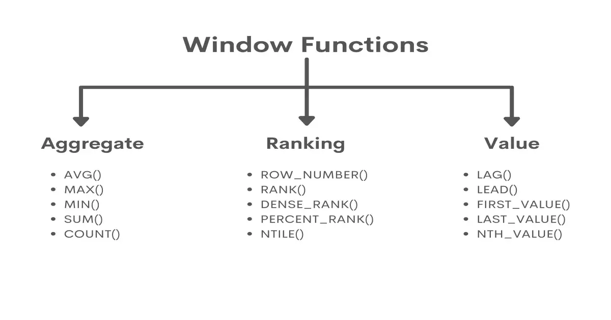
Window functions are an advanced type of function that allows us to perform calculations across a set of table rows that are somehow related to the current row, returning a single value for each row.
What is a window?
A window consists of a group of rows that are related in some way. The relation could be by location (e.g. city), time (e.g. days, month), or that they happen to be in the same result set. Calculations are made over this subset of data.
Simple Window Function
The OVER() clause must be used to create a basic window function. By default, this will treat the entire result set as a single partition if no parameters are provided.
I have created a dataset in Snowflake for testing the below queries. You may need to adapt these to make them compatible with your DBMS. The dataset contains the volume of three retail locations, across three days and two cities.
Create The Dataset:-- Create Table
CREATE TRANSIENT TABLE store_sales (
store_ID INTEGER,
day INTEGER,
city VARCHAR,
gross_sales NUMERIC(9, 2)
);
-- Insert Data
INSERT INTO store_sales VALUES
(1, 1, 'London', 100),
(1, 2, 'London', 123),
(1, 3, 'London', 67),
(2, 1, 'Manchester', 738),
(2, 2, 'Manchester', 673),
(2, 3, 'Manchester', 523),
(3, 1, 'London', 642),
(3, 2, 'London', 673),
(3, 3, 'London', 512);
Let's perform as regular SUM() aggregation where Day = 1. This returns 1,480 total gross sales across the dataset.
Results:SELECT SUM(GROSS_SALES) AS total_sales FROM store_sales WHERE day = 1We want to know what stores contributed the most to this figure. This is a perfect use case for using a window function. We can add the “OVER()” clause to our SUM() to create a window across the result set. Now each row also contains the total gross_sales across the result set. We can use this to show each row's contribution to the total gross sales as a percentage.
SELECT store_ID, day, city, gross_sales, SUM(gross_sales) OVER() AS total_sales, gross_sales / SUM(gross_sales) OVER() AS sales_contribution FROM store_sales WHERE day = 1
| # | STORE_ID | DAY | CITY | GROSS_SALES | TOTAL_SALES | SALES_CONTRIBUTION |
|---|---|---|---|---|---|---|
| 1 | 1 | 1 | London | 100 | 1480 | 0.06756757 |
| 2 | 2 | 1 | Manchester | 738 | 1480 | 0.49864865 |
| 3 | 3 | 1 | London | 642 | 1480 | 0.43378378 |
PARTITON BY Clause
The PARTITION_BY clause allows us to split the results set into partitions. The window function is applied to each partition separately, with the computations restarting for each partition. If no PARTITION_BY is specified, the function treats all rows of the query result set as a single partition (as seen previously).
We are able to calculate the total gross_sales by city, and also calculate which stores contributed the most to the gross sales for each city.
SELECT
    store_ID,
    day,
    city,
    gross_sales,
    SUM(GROSS_SALES) OVER(PARTITION BY city) AS total_sales,
    gross_sales / SUM(GROSS_SALES) OVER(PARTITION BY city) AS totasales_contribution
FROM store_sales
WHERE
    day = 1
| # | STORE_ID | DAY | CITY | GROSS_SALES | TOTAL_SALES | SALES_CONTRIBUTION |
|---|---|---|---|---|---|---|
| 1 | 1 | 1 | London | 100 | 742 | 0.13477089 |
| 2 | 2 | 1 | Manchester | 738 | 738 | 1.00000000 |
| 3 | 3 | 1 | London | 642 | 741 | 0.86522911 |
ORDER BY Clause
The ORDER BY clause defines the logical order of the rows within each partition. If this has not been, defined the default order is ascending. Some queries and functiosn are can be order-sensitive and are dependent on the order of the rows.
Types of order sensitive window functions:
- Rank-Related Window Functions
- Window Frame Functions
Rank-Related Window Functions
Rank realted window functions provide a rank which is the order of a row in an ordered window of rows. The first row in the window has rank 1, the second rank 2, etc. Rank doesn’t automatically sort the rows, so the ORDER BY sub clause must be used.
ROW_NUMBER() allows us to return a unique number for all rows, sequentially. Even if two rows have the same value, they will still be sequentially numbered.
RANK() works similar to ROW__NUMBER(), but will provide the same numeric values for ties. This can leave a gap in the ranking. DENSE_RANK() works similar to RANK(), but with no gaps in the ranking values. The row value is the rank of a specific row, plus the number of distinct rank values that come before that specific row.
SELECT
   store_id,
   day,
   city,
   gross_sales,
   ROW_NUMBER() OVER (ORDER BY gross_sales DESC) ROW_NUMBER,
   RANK() OVER (ORDER BY gross_sales DESC) RANK,
   DENSE_RANK() OVER (ORDER BY gross_sales DESC) DENSE_RANK
FROM store_sales| # | STORE_ID | DAY | CITY | GROSS_SALES | ROW_NUMBER | RANK | DENSE_RANK |
|---|---|---|---|---|---|---|---|
| 1 | 2 | 1 | Manchester | 738.00 | 1 | 1 | 1 |
| 2 | 2 | 2 | Manchester | 673.00 | 2 | 2 | 2 |
| 3 | 3 | 2 | London | 673.00 | 3 | 2 | 2 |
| 4 | 3 | 1 | London | 642.00 | 4 | 4 | 3 |
| 5 | 2 | 3 | Manchester | 523.00 | 5 | 5 | 4 |
| 6 | 3 | 3 | London | 512.00 | 6 | 6 | 5 |
| 7 | 1 | 2 | London | 123.00 | 7 | 7 | 6 |
| 8 | 1 | 1 | London | 100.00 | 8 | 8 | 7 |
| 9 | 1 | 3 | London | 67.00 | 9 | 9 | 8 |
Window Frame Functions
A window frame is a sub-group of rows in a window, allowing you to compute values over the sub-group of rows rather than over the entire window.
There are two types of window frames:
- Cumulative
- Sliding
These can be calculated using the ROWS BETWEEN clause to specify the lower (starting) and upper (ending) boundary points of the window frame. This is placed after the ORDER BY clause.
The syntax: ROWS BETWEEN <window frame bound> AND <window frame bound>.
UNBOUND PRECEDING: Specifies that the window starts at the first row of the partition. This can only be specified as the lower boundary of a window frame. You can define the start point using “<value> PRECEDING”. E.g. “2 PRECEDING”
CURRENT ROW: Specifies that the window frame starts or ends at the current row and can be specified as both the start and end point.
UNBOUNDED FOLLOWING: Specifies that the window ends at the last row of the partition. This can only be specified as the upper boundary of a window frame. You can define the starting point using "<value> FOLLOWING". E.g. "2 FOLLOWING" defines a window ending with the second row that follows the current row.
Cumulative Window Fram
A cumulative window frame is a variable-width window that starts at a fixed point and grows with each row. An example of this is using daily data to calculate the total gross_sales for a month. A cumulative window frame will start on the first day of the month and grow as each new day's data is added.
Example of a cumulative window function by store and month, calculating the cumulative sales leading to the end of the month:
SUM(gross_sales) OVER (PARTITION BY STORE_ID, Month ORDER BY DAY ROWS BETWEEN UNBOUNDED PRECEDING AND CURRENT ROW)Sliding Window Frame
You can define a fixed-width frame that “slides along” the rows in the window, showing you a different slice of the window each time. As the window frame moves along the data, old rows disappear from the frame and new rows appear so that the width of the frame is always the same.
This is useful for calculating moving aggregations (calculated using a fixed-size interval that moves). The below example will give the total gross sales for the previous 11 months, and the current month.
SUM(gross_sales) OVER (PARTITION BY STORE_ID ORDER BY MONTH ROWS BETWEEN 11 PRECEDING AND CURRENT ROW)If your data is already aggregated by month, you could produce a 12-month rolling average using:
AVG(gross_sales) OVER (PARTITION BY STORE_ID ORDER BY MONTH ROWS BETWEEN 11 PRECEDING AND CURRENT ROW)Filtering the results of window functions
To filter the results of a window function you will need nest the query and filter it.
Filtering using nesting:
SELECT *
    FROM (
        SELECT x, y, z
        ROW_NUMBER() OVER (PARTITION BY x ORDER BY z) AS row_num
    FROM qt
)
WHERE row_num = 1
Snowflake introduced the QUALIFY clause, simplifying the filtering process on the result of window functions.
Filtering using QUALIFY:
SELECT x, y, z
FROM qt
QUALIFY ROW_NUMBER() OVER (PARTITION BY x ORDER BY z) = 1